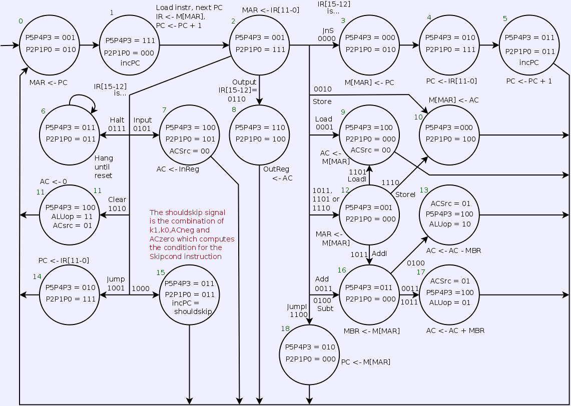
The behavior of the Marie controller can be described by the following state diagram. Each state represents one clock period, and the controller will output the signal shown in the circles. Boolean signals which are not listed are false; others are don't-care. States are numbered arbitrarily. The controller starts in state 0, and changes to another state at the end of each clock period. Some changes depend on the op code, but most do not.
Note that this implements a slightly different RTL than that given in Table 4.7 and in the main notes. Null & Lobur (almost) always move data between memory and the MBR, even though the datapath, both in Fig. 4.9 and in my Logisim solution, connects the memory data port to the main bus, so it can be sent or received from anywhere. This adds extra steps to most of the non-trivial instructions. They also use their PC increment unit during the initial instruction fetch, and for Skipcond, but not for JnS. The versions here use fewer cycles, and require fewer states in the state machine.
JnS X [changed]
M[MAR] ← PC PC ← X PC ← PC + 1
Load X [changed]
MAR ← X AC ← M[MAR]
Store X [changed]
MAR ← X, M[MAR] ← AC
Add X
MAR ← X MBR ← M[MAR] AC ← AC + MBR
Subt X
MAR ← X MBR ← M[MAR] AC ← AC - MBR
Input
AC ← InREG
Output
OutREG ← AC
Skipcond
If IR[11-10] = 00 then If AC < 0 then PC ← PC + 1 else if IR[11-10] = 01 then If AC = 0 then PC ← PC + 1 else if IR[11-10] = 10 then If AC > 0 then PC ← PC + 1
Jump X
PC ← IR[11-0]
Clear
AC ← 0
AddI X [changed]
MAR ← X MAR ← M[MAR] MBR ← M[MAR] AC ← AC + MBR
JumpI X [changed]
MAR ← X PC ← M[MAR]
LoadI X [changed]
MAR ← X MAR ← M[MAR] AC ← M[MAR]
StoreI X [changed]
MAR ← X MAR ← M[MAR] M[MAR] ← AC