Array Location Arithmetic

[Ch. 1: Overview and History] [Syntax] [Names and Scope] [Types and Type Systems] [Semantics] [Functions] [Memory Management] [Imperitive Programs and Functional Abstraction] [Modular and Class Abstraction] [Functional Programming] [Logic Programming]

[Type Propagation] [Array Location Arithmetic]

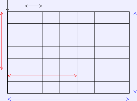
Arrays are typically layed out continguously in memory. The basic parameters are:

α The starting address of the array.

e The size of an array element.

lb, ub The lower and upper array bounds.

a[i] The subscript expression being evaluated.

So, for a one-dimensional array,

a[i]

a[lb..ub]

i-lb slots

The address of address of the location a[i] is given by:

addr(a[i]) = α + e(i − lb) = (α − e⋅lb) + e⋅i

This can be generalized for a two-dimensional array. Note that the first cell of each row is located in memory just after the last cell of the row above it.

a[i,j]

a[lb1..ub1, lb2..ub2]

i−lb1
rows

j−lb2 slots

ub1−lb1 + 1 rows

ub2−lb2 + 1 columns

So the address of a[i] will be given by starting from α and first skipping the rows above it, then the cells to its left.

addr(a[i,j]) = α + e(ub2−lb2+1)(i−lb1) + e(j−lb2)
= (α − e⋅ub2⋅lb1 + e⋅lb2⋅lb1 − e⋅lb1 − e⋅lb2) + i(e⋅ub2 − e⋅lb2 + e) + e⋅j

Languages which create multi-dimensional arrays as shown here typically require that the bound be constants. That means that the address formulas can be reduced at compile to time to a linear computation of the subscripts (the sum of a constant and a constant multiple of each subscript).

In languages like C and Java, where the lower bound is zero, and the upper bound is the size less 1, we can substitute 0 for each lb and s−1 for each ub and get:

addr(a[i]) = α + ei

addr(a[i,j]) = α + s2⋅e⋅i + e⋅j

α	The starting address of the array.
e	The size of an array element.
lb, ub	The lower and upper array bounds.
`a`[`i`]	The subscript expression being evaluated.