1. Transmission of data by some physical means.
   1. Physics. Describe and predict the behavior of a signal crossing some physical medium.
   2. Mathematics. How to best represent the data using measurable physical quantities.
   3. Engineering. Effectively realize the the schemes, i.e., make it actually work, and at an affordable cost.
   4. Several steps may be involved.
      1. Information sources may be digital or analog. In the later case, source encoding must include some sort digital conversion.
      2. Encryption is used to secure against snooping, and can be omitted if that is not an issue.
      3. Chanel encoding usually includes some method for the decoder to detect errors.
      4. Multiplexing refers to the sending of multiple signals sharing a single channel.
   5. Not all steps are needed in every case (or some may be trivial).
2. Signals
   1. Measurable energy.
   2. Analog and digital.
      
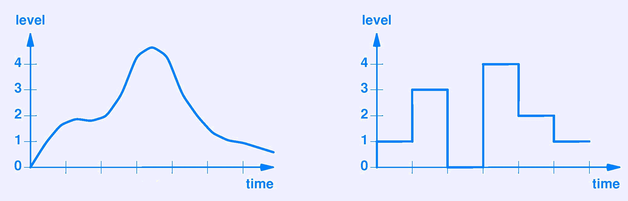
   3. Periodic or aperiodic.
3. Sine waves
   1. A very important kind of periodic signal described by the sine function.
      1. Amplitude: The height of curve maximum.
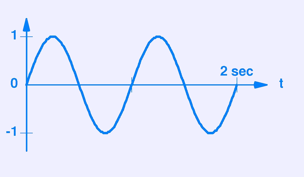
      2. Frequency: The number of cycles per second.
      3. Phase: The delay of the start of the first complete cycle from some reference time.
      

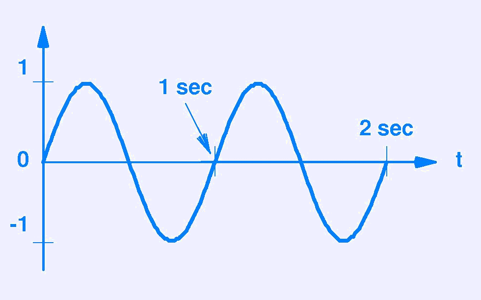      sin(2πt)

      

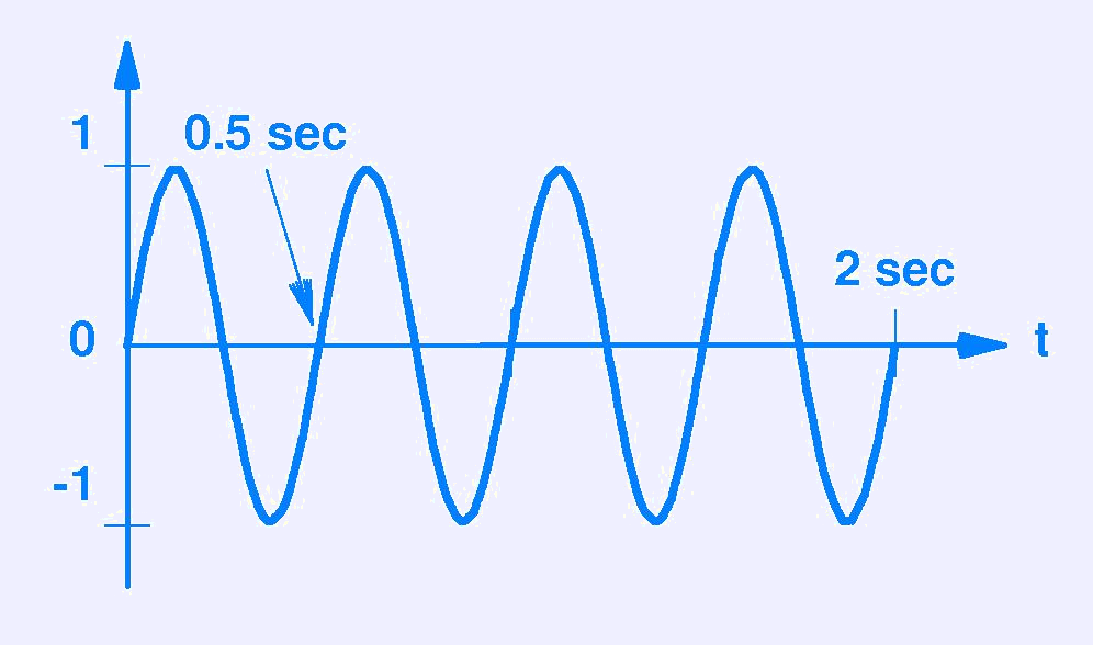      Higher frequency: sin(2π2t)

      

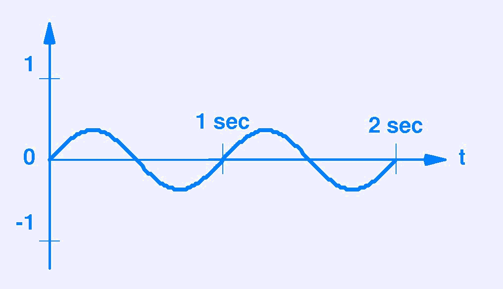      Lower amplitude: 0.4sin(2πt)

      

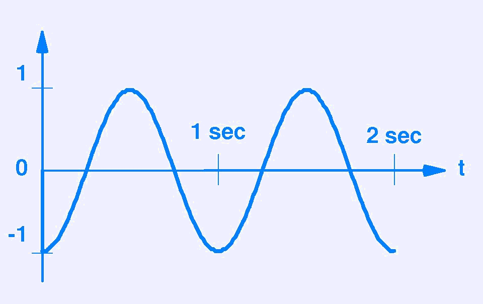      Phase change: sin(2πt+1.5π)
   2. Many natural phenomena produce sinusoidal signals.
   3. Sine waves tend to survive transmission better than digital signals.
4. Combining sine waves.
   1. Sine waves may be combined to form more complex signals.
      

      sin(2πt)

      

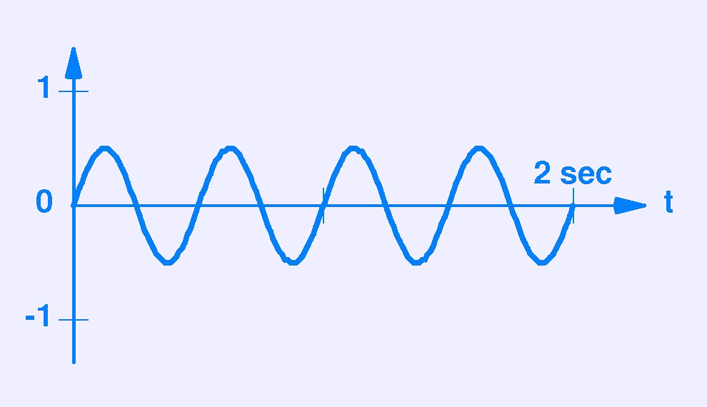      0.5sin(2π2t)

      

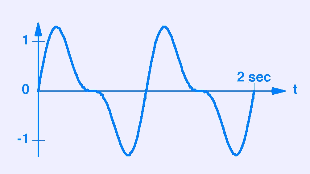      sin(2πt)+0.5sin(2π2t)
   2. Fourier discovered how to decompose any signal into a sum of sine waves.
   3. The curves above represent the signal in the “time domain,” as a function from time to signal strength (voltage, etc.)
   4. They can also be represented in the “frequency domain,” as a function from frequency to amplitude. The sum from above is:
      
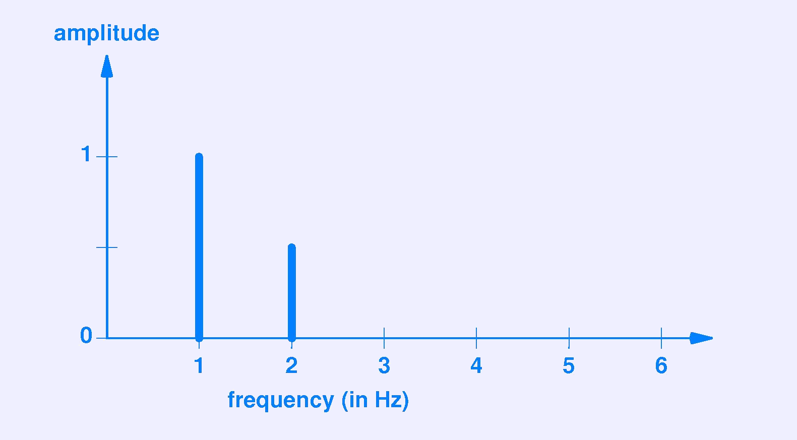
   5. The Fourier transform is essentially a function from one function to another.
      1. By convention, f is the time-domain function, and F is the frequency-domain.
      2. Notation: ℱ{f(t)}=F(s) ℱ−1{F(s)}=f(t)
      3. The transform is 1:1, so any signal has essentially two forms.
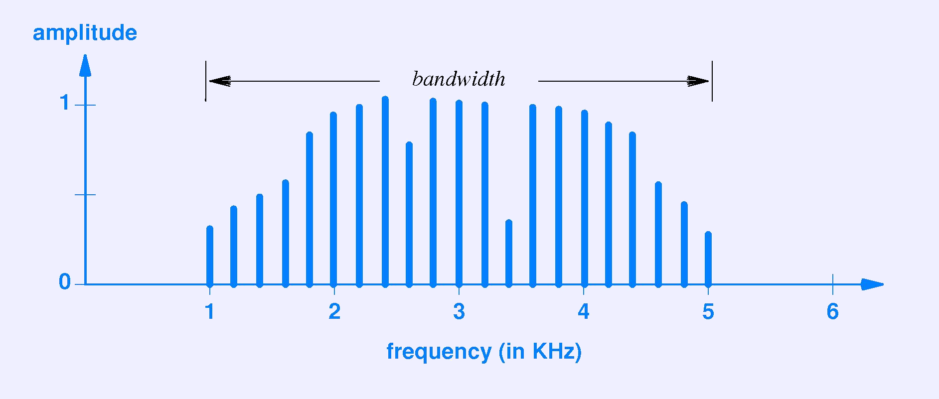
   6. The bandwidth of an analog signal is the range of frequencies present.
      
5. Sending digital data.
   1. You can data faster by using more levels.
      
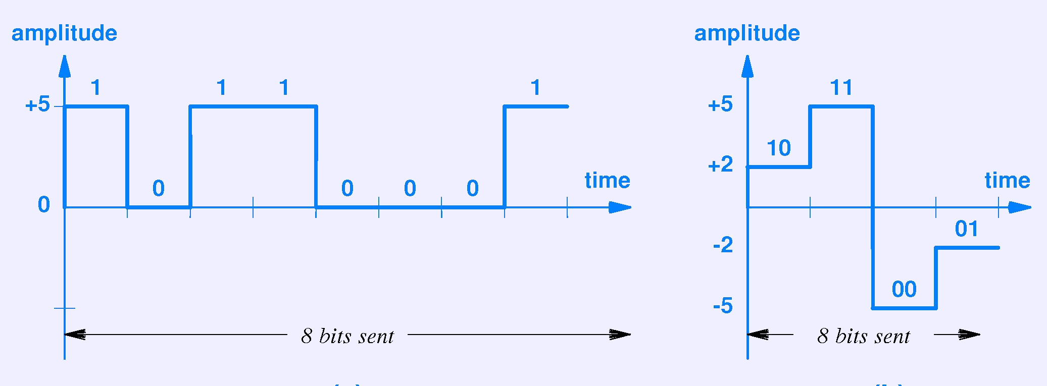
   2. Using n levels, you can send log2n bits at a time.
   3. Why can't we just use 10000 levels and just rush it through?
      1. Must be far enough apart for the receiver to tell which.
      2. In practice, you can only have a few levels.
   4. You can send data faster by holding each symbol a shorter time.
   5. So why can't we just hold each one for a ns and rush it through?
      1. Must stay long enough for the receiver to notice.
      2. The maximum rate at which the changes can be detected is called the baud rate.
   6. For n levels over a digital channel with baud rate b, the data rate d, in bits per second is:
      d=b⌊log2n⌋
   7. Of course, the endpoints must agree on the number and assignment of levels, bit time, and many other details.
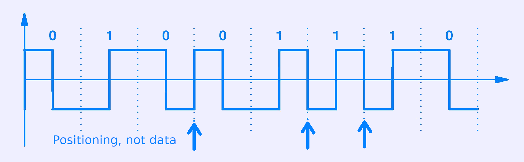
6. Line Coding. How to represent the bits in the signal.
   1. Common to assign bits to changes rather than levels. Faster to detect.
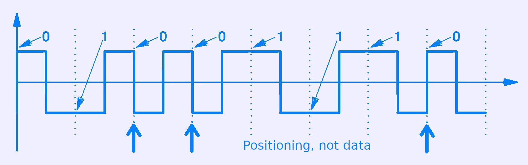
   2. Manchester encoding.
      1. Bits are recognized in the middle of a bit period.
      2. Upward transition is 1
      3. Downward transition is a 0.
      4. To send repeats, an extra transition is performed to get ready.
      
      
   3. Differential Manchester
      1. Bits are still recognized in the middle of a bit period.
      2. A transition in the opposite direction from the last is a 1.
      3. A transition in the same direction from the last is a 0.
      4. Extras are needed to send zeros.
      
      
   4. NRZ-I. The signal changes for one bits and stays the same for zero.
      
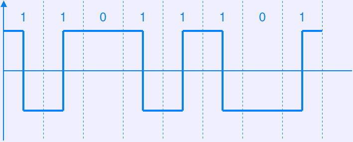
   5. Changes tell the receiver when the sender thinks bit periods start and end. NRZ-I needs some extra synchronization mechanism if it must send a long run of zeros.
7. Digitizing analog sources.
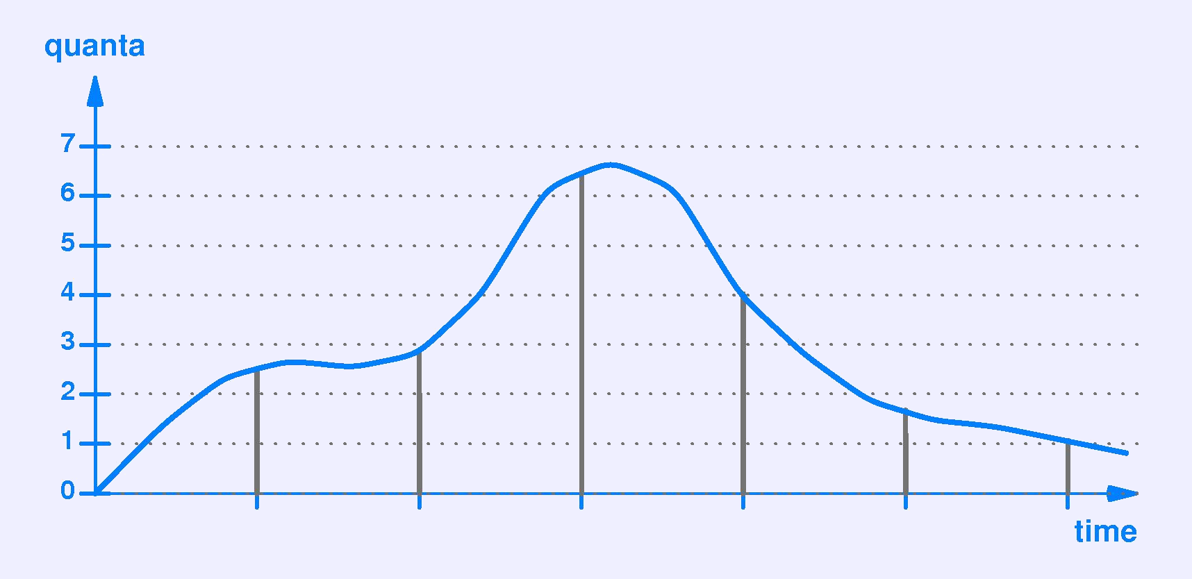
   1. Periodically sample (measure) the value of the analog signal. Result is a series of measurements.
      
   2. Sometimes take multiple measurements (three say), and report the mean of each. Reduces transient distortions.
   3. “Pulse-Code Modulation”: Report the measurements.
   4. “Delta Modulation”: Report the first measurement, then differences.
      1. Differences are smaller, use less space.
      2. Suffers more from transmission errors.
   5. Sampling
      1. Larger sample size is more accurate, but generates more data.
      2. More frequent sampling is more accurate, but generates more data.
      3. Nyquist Theorem: Sample at twice the highest frequency you wish to retain: two samples for each wave.
         1. Follows from the fact that the signal is the sum of sine waves.
         2. If you have y=Asin(2πft), two points within the same cycle determine f and A.
      4. Traditional telephone sampling.
         1. 4000 Hz audio quality.
         2. 8-bit samples (0-255).
         3. Voice call: 8000samples/second×8bits/sample=64000bits/second
      5. CD music: 44100 Hz. Sound a lot better.
   6. Encoding.
      1. Linear: Simply record the measurement.
      2. Non-linear: The numbers are transformed to reduce the range of values so they code more effectively.
      3. US standard called μ-law; Euro called a-law.
   7. Compression is also possible, lossless (classical), or lossy.